Bayes Factors and Meta-Analysis

Preface

This is a short exploration on why Bayes Factors are not a good idea when conducting a meta-analysis. I will demonstrate a very simple example of how prior selection can practically eliminate the ability for a Bayes Factor to make sense.

If you are extremely familiar with Bayesian analysis and hypothesis testing, the ending may be spoiled. This was unfortunately something I encountered myself (made a bit of a fool of myself in a meeting to boot) because as far as my education up to that point in time could inform me, Bayes Factors were how my research group would be able to tell more about our results and evaluate evidence for or against our null and alternative hypotheses. And, most of the literature I had encountered until that point merely said there were reasons to be cautious when using Bayes factors - just sort of a general warning. Here is another warning, I suppose, with an example.

An Example with Multple Sclerosis Treatments

For the sake of example, I take a dataset from a previous meta-analysis and then replicate their results with a Bayesian random effects meta-analysis in the R package brms.¹ Then, I use bayestestR to provide a summary of the subsequent posterior distribution. This is pretty standard workflow when modelling, and I mostly provide another example of this in another set of notes on Bayesian Meta-analysis.

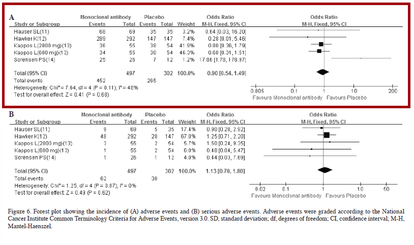
The example study by Xie et al. includes 4 studies with over 745 individuals pooled together.¹ In the study, they used frequentest methods (the DerSimonian and Laird default in RevMan), and we should be able to replicate their results with a Bayesian version to a satisfactory degree. They examined the pooled relationship between monoclonal antibody type anti-B-cell treatments (Rituximab, Ocrelizumab and Ofatumumab in this case) and a number of adverse outcomes.

We only need to focus on one of their meta-analyses to get the point across, but feel free to go back and do more. I am going to focus on the analysis they conducted examining any adverse event across studies that they show in Figure 6, which for reference looks like this:

Let’s replicate the results from Forest plot A - any adverse events. We’ll expect a slightly protective effect, with dubious practical significance. Also, we will assume that we can use the confidence limits to estimate study variance using:

$$\begin{gathered} \log (\text{OR})\pm 1.96\cdot {\text{SE}}_{\log (\text{OR})} \\ \Rightarrow {\text{SE}}_{\log (\text{OR})}=\frac{\log (\text{UCL})-\log (\text{LCL})}{2\times 1.96} \end{gathered}$$

#load packages
library(tidyverse)
library(gt)

# recreate dataset for use:
ORs <- c(0.64, 0.28, 0.80, 0.68, 17.86)
LCL <- c(0.03, 0.01, 0.36, 0.31, 1.78)
UCL <- c(16.2, 5.46, 1.79, 1.51, 178.97)
n   <- c(104, 439, 109, 109, 38)
name <- c("Hauser et al.", "Hawker et al.", "Kappos et al.", "Kappos et al.", "Sorensen et al.")



# Create data frame from raw input
data <- data.frame(
  Study = name,
  N = n,
  OR = ORs,
  LCL = LCL,
  UCL = UCL
)

# Add derived columns
data <- data %>%
  mutate(
    CI = paste0("[", sprintf("%.2f", LCL), ", ", sprintf("%.2f", UCL), "]"),
    logOR = log(OR),
    SE_logOR = (log(UCL) - log(LCL)) / (2 * 1.96)
  )

# Make gt table
data %>%
  gt() %>%
  tab_header(
    title = "Study Data for Meta-Analysis",
    subtitle = "from Figure 6.A"
  ) %>%
  fmt_number(columns = c(OR, logOR, SE_logOR), decimals = 2) %>%
  cols_label(
    Study = "Study (First Author)",
    N = "n",
    OR = "Odds Ratio",
    CI = "95% CI",
    logOR = "log(OR)",
    SE_logOR = "log(SE)"
  )

Study Data for Meta-Analysis
from Figure 6.A
Study (First Author)	n	Odds Ratio	LCL	UCL	95% CI	log(OR)	log(SE)
Hauser et al.	104	0.64	0.03	16.20	[0.03, 16.20]	−0.45	1.60
Hawker et al.	439	0.28	0.01	5.46	[0.01, 5.46]	−1.27	1.61
Kappos et al.	109	0.80	0.36	1.79	[0.36, 1.79]	−0.22	0.41
Kappos et al.	109	0.68	0.31	1.51	[0.31, 1.51]	−0.39	0.40
Sorensen et al.	38	17.86	1.78	178.97	[1.78, 178.97]	2.88	1.18

Log Odds Ratio

If you are wondering why I am using log(OR) instead of just the OR itself, please consider checking my other notes on meta-analysis with Bayesian methods, or see some of the sources I mention, e.g. the Handbook of Meta-Analysis.²

Now, we just plug in that information into a meta-analysis model. I’m going to use a random effects model, which may be solid choice due to the clear heterogeneity between studies. I’ll go ahead and show the code here too, so you can also try.

I’m choosing vague priors here that I’ve seen commonly in examples of meta-analysis: intercept/effect – normal(0, 1000), and heterogeneity – lognormal(0, 0.5). It’s quite a vague prior for the effect, so that I am not overwhelming the four observations when it comes to prior vs. likelihood.

# packages used
library(brms)
library(bayestestR)


model <- brm(
  formula = logOR | se(SE_logOR) ~ 1 + (1 | Study),  
  data = data,
  family = gaussian(),
  prior = c(
    prior(normal(0, 1000), class = Intercept),
    prior(lognormal(0, 0.5), class = sd)
  ),
  iter = 4000,
  warmup = 1000,
  chains = 4,
  cores = 4,
  seed = 123
)

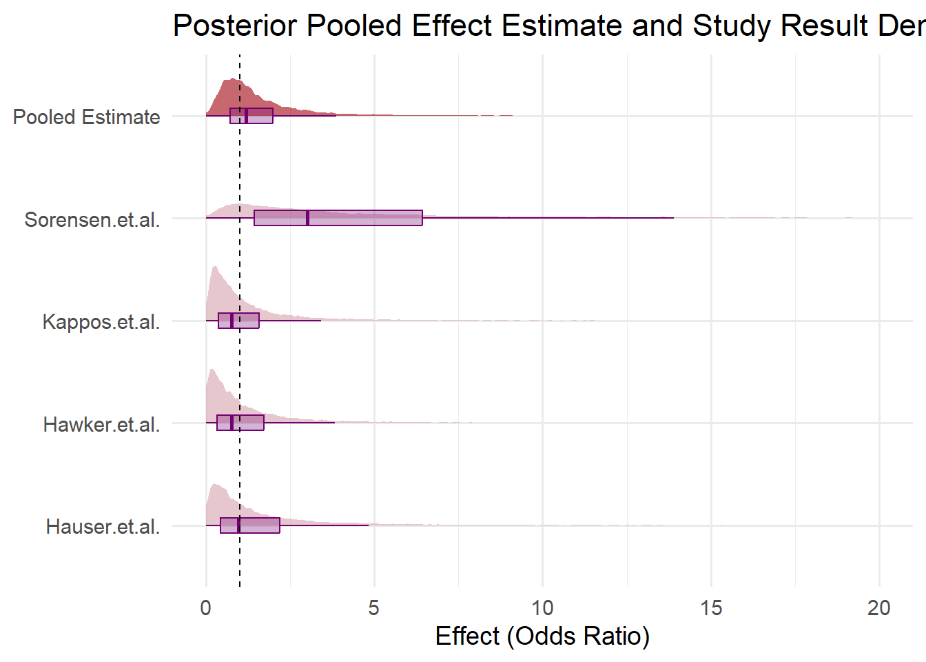
Here I create a blobbogram to visualize the estimated prior sampling at the top in red, box plots with the median as the central mark in purple, and the simulated distributions from the results of the studies used in the meta-analysis.

library(tidybayes)

# posterior draws for our overall effect
pooled_draws <- as_draws_df(model) %>%
  select(b_Intercept) %>%
  mutate(
    Study = "Pooled Estimate",
    logOR = b_Intercept,
    OR = exp(logOR)
  ) %>%
  select(Study, OR)

# Extract posterior draws for random effects by study
# Note: brms names random effects like r_Study[StudyName,Intercept]
study_draws_raw <- as_draws_df(model) %>%
  select(starts_with("r_Study")) 

# Tidy the random effects draws to long format
study_draws <- study_draws_raw %>%
  pivot_longer(cols = everything(),
               names_to = "param",
               values_to = "random_effect") %>%
  mutate(
    # Extract study names from param string
    Study = str_extract(param, "(?<=r_Study\\[)[^,]+"),
    # Add the fixed intercept to random effect for full logOR posterior per study
    logOR = random_effect + as_draws_df(model)$b_Intercept,
    OR = exp(logOR)
  ) %>%
  select(Study, OR)

# Combine pooled and study-specific draws
plot_data <- bind_rows(
  study_draws,
  pooled_draws
)

# Make sure "Pooled Estimate" is last for plotting order
plot_data$Study <- factor(plot_data$Study, levels = c(sort(unique(study_draws$Study)), "Pooled Estimate"))

# Plot raincloud (half-eye + boxplot + jitter) using ggdist
ggplot(plot_data, aes(x = Study, y = OR, fill = (Study == "Pooled Estimate"))) +
  stat_halfeye(
    adjust = 0.5, width = 0.6, .width = 0.95, slab_alpha = 0.6, point_interval = NULL) +
  geom_boxplot(width = 0.15, outlier.shape = NA, alpha = 0.3, fill = "#730071", color = "#730071") +
  #geom_jitter(width = 0.1, alpha = 0.2, size = 0.5) +
  scale_fill_manual(values = c("TRUE" = "#A0030B", "FALSE" = "#D6A2AD"), guide = "none") +
  geom_hline(yintercept = 1, linetype = "dashed") +
  coord_flip() +
  scale_y_continuous(limits = c(0, 20)) +
  labs(
    title = "Posterior Pooled Effect Estimate and Study Result Densities",
    x = NULL,
    y = "Effect (Odds Ratio)"
  ) +
  theme_minimal(base_size = 14)

This looks a lot like what the previous authors found at first glance. However, it’s pretty clear we’re estimating a harmful relationship (OR > 1) between any adverse event and the treatments. The long tail of our posterior appears to have pulled our median estimate into the positive, even thought the mode appears to be between 0 and 1. In the output from describe_posterior() below, we see the estimate is an odds ratio of about 1.2. However, in both our analysis and the results in the example study, we may not have a lot of information to determine any real difference. Xie et al. include a wide confidence interval, and we have a wide credible interval - these can’t be directly compared but both suggest low precision. Small wonder, with only four observations.

Additionally, thanks to our Bayesian analysis, we can say that the probability that the OR is protective (less than 1):

#calculate the probability the value is less than 1:
p_0.9 <- pooled_draws %>%
  filter(OR < 1) %>%
  nrow() / nrow(pooled_draws)

That’s a probability of just over 0.4 - still a large percentage based on our model! Its too close to a coin flip for my confidence in treatments being protective or harmful for any adverse event, and leaving an estimate of 0.9 being probable enough to make me distrustful.

In any case, we can’t really tell if the odds of experiencing any adverse event is greater in those with or without anti-B-Cell treatments based on these few studies. Good thing there were plenty more studies done after 2017.

The Beef with BF

The model appears to be working, our estimates make sense, so let us examine our hypotheses with a typical Bayes Factor. I’ll use bayestestR here to generate the usual percentage of the posterior out side of the region of practical equivalence (ROPE%), the probability of direction (PD), and of course the Bayes Factor:

#packages
library(bayestestR)

# Extract posterior draws of the overall effect (logOR)
post_raw <- as_draws_df(model)$b_Intercept
post <- exp(post_raw)
prior <- rnorm(length(post), mean = 0, sd = 1000)

bf_result <- bayesfactor_parameters(
  posterior = post,
  prior = prior,
  null = 0
)

# Compute ROPE percentage (choose a reasonable practical equivalence range)
summary_stats <- describe_posterior(post, rope_range = c(0.9, 1.1))
bf <- bayesfactor_parameters(posterior = post, prior = prior, null = 0)
summary_stats$BF <- exp(bf$log_BF)
summary_stats$pd <- as.numeric(p_direction(post, null = 1))

# Combine into a clean gt table
summary_stats%>%
  select(Parameter, Median, CI_low, CI_high, pd, ROPE_Percentage, BF) %>%
  mutate(across(where(is.numeric), ~ round(.x, 2))) %>%
  gt() %>%
  tab_header(
    title = "Posterior Summary for Overall Effect (logOR)",
    subtitle = "Including pd and % in ROPE"
  ) %>%
  cols_label(
    CI_low = "Lower 95% CrI",
    CI_high = "Upper 95% CrI",
    pd = "Probability of Direction",
    ROPE_Percentage = "% in ROPE",
    BF = "Bayes Factor"
  )

Posterior Summary for Overall Effect (logOR)
Including pd and % in ROPE
Parameter	Median	Lower 95% CrI	Upper 95% CrI	Probability of Direction	% in ROPE	Bayes Factor
Posterior	1.19	0.23	6.2	0.6	0.12	0.03

We can see that the BF suggests evidence for the alternative is extremely weak, our probability of direction is low, and even though the % rope is not too bad, this seems like we overall have no statistical evidence to suggest there is an effect from our treatments on combined adverse events in these studies. The BF unfortunately makes sense.

However, other vague priors might also make sense to us, if we don’t have prior knowledge. If we change the effect prior to examine the changes in the Bayes factor, (say from normal(0,1000) to normal(0,10), potentially reasonable since we don’t expect a standard error of 1000 in reality) things cease to make sense. Now the BF suggests that the alternative hypothesis is 13 times more likely than the null. This is still with a vague prior, just assuming less variance. We get the following output:

model <- brm(
  formula = logOR | se(SE_logOR) ~ 1 + (1 | Study),  
  data = data,
  family = gaussian(),
  prior = c(
    prior(normal(0, 10), class = Intercept),
    prior(lognormal(0, 0.5), class = sd) 
  ),
  iter = 4000,
  warmup = 1000,
  chains = 4,
  cores = 4,
  seed = 123
)


# Repeat summary from before
post_raw <- as_draws_df(model)$b_Intercept
post <- exp(post_raw)
prior <- rnorm(length(post), mean = 0, sd = 1000)

bf_result <- bayesfactor_parameters(
  posterior = post,
  prior = prior,
  null = 0
)

# Compute ROPE percentage
summary_stats <- describe_posterior(post, rope_range = c(0.9, 1.1))
bf <- bayesfactor_parameters(posterior = post, prior = prior, null = 0)
summary_stats$BF <- exp(bf$log_BF)
summary_stats$pd <- as.numeric(p_direction(post, null = 1))

# Combine into a clean gt table
summary_stats%>%
  select(Parameter, Median, CI_low, CI_high, pd, ROPE_Percentage, BF) %>%
  mutate(across(where(is.numeric), ~ round(.x, 2))) %>%
  gt() %>%
  tab_header(
    title = "Posterior Summary for Overall Effect (logOR)",
    subtitle = "Including pd and % in ROPE"
  ) %>%
  cols_label(
    CI_low = "Lower 95% CrI",
    CI_high = "Upper 95% CrI",
    pd = "Probability of Direction",
    ROPE_Percentage = "% in ROPE",
    BF = "Bayes Factor"
  )

Posterior Summary for Overall Effect (logOR)
Including pd and % in ROPE
Parameter	Median	Lower 95% CrI	Upper 95% CrI	Probability of Direction	% in ROPE	Bayes Factor
Posterior	1.2	0.24	6.79	0.6	0.11	13.06

Of course one should always check priors and use caution when deciding which distribution and parameters. However, the BF quickly becomes nonsense. The estimates for everything except the BF remain nearly the exact same thing same - our posterior really didn’t change. So what happened? How can we reconcile the BF to the ROPE% - both of which are supposed to help in hypothesis testing?

The Main Point

As demonstrated, the Bayes Factor is unstable in meta-analysis due to the low number of observations, and can easily be misleading.

In general, Bayes Factors should be used cautiously, and the interpretation of them as being the probability of a hypothesis being accurate compared to another is oversimplified.

How this happens mathematically has been previously outlined by van der Linden et al.³ As they put it, “Bayes factors provide an incoherent framework for evidential support because of their high sensitivity to the prior and because the penalize hypotheses that contain values with low likelihoods.” They also cite other works that have further discussion of Bayes Factors, like a fun article from Lavine and Schervish.⁴ There is also a mention of the issue in chapter 7 of Bayesian Data Analysis.⁵

A simple explanation can be provided by examining the definition of a Bayes Factor, as we use it for null versus alternate hypothesis testing:

$$BF=\frac{\left[\frac{p(M=null|D)}{p(M=alt|D)}\right]}{\left[\frac{p(M=null)}{p(M=alt)}\right]}$$ Where $D$ is the observed data, and $M$ is the index of probability between null and alternate.⁶ The Bayes Factor works by examining the change in probability of null vs. alternate (via $M$ here), across the change in prior to posterior. See Kruschke & Liddell for more information.⁶ They mention the exact issue I want to highlight in these notes towards the end of their article - and suggest that instead of looking at Bayes Factors, one should examine the precision of the study and determine if that was reasonable. That is more informative because the index $M$ has a bit of an obscured effect on the BF that is apparently easily overlooked. If only I knew earlier that my prior education omitted this article and the concept within it.

So, remember - A Bayes Factor is a change in support for a hypothesis when moving from prior to posterior, relative to another hypothesis.⁴ Because of that, they can be confusing in certain situations and reinforce the need for critical thinking in prior selection, and aren’t just how much more likely one hypothesis is than another.

Postface

I feel like this is a it too simple of an explanation, but unfortunately time is short and these are just field notes I’m volunteering to the world. I hope this adds a bit of further understanding of how Bayesian analysis is best applied, and if you have more questions about null hypothesis testing in Bayesian analysis, I emphasize again the source mentioned earlier - Kruschke & Liddell.⁶ For additional discussion of the goals of Bayesian analysis on a broader sense, I would suggest reading Gelman and Shalizi’s “Philosophy and the practice of Bayesian statistics” in the 66th issue of the British Journal of Mathematical and Statistical Psychology from 2013.⁷ It’s a thought-provoking paper that focuses more on the application of Bayesian model checking vs. Bayesian updating within the scientific process.

AI Disclaimer

Some of the code used was written with the help (or hindrance) of ChatGPT.

References

1.

Xie Q, Li X, Sun J, et al. A meta‑analysis to determine the efficacy and tolerability of anti-b-cell monoclonal antibodies in multiple sclerosis. Experimental and Therapeutic Medicine. 2017;13:3061-3070. doi:10.3892/etm.2017.4298

2.

Schmid CH, Stijnen T, White IR, eds. Handbook of Meta-Analysis. CRC Press; 2021. https://www.crcpress.com/Chapman--HallCRC-Handbooks-of-Modern-Statistical-Methods/book-series/CHHANMODSTA

3.

Linden S van der, Chryst B. No need for bayes factors: A fully bayesian evidence synthesis. Frontiers in Applied Mathematics and Statistics. 2017;3:12. doi:10.3389/fams.2017.00012

4.

Lavine M, Schervish MJ. Bayes factors: What they are and what they are not. The American Statistician. 1999;53(2):119-122. doi:10.1080/00031305.1999.10474443

5.

Gelman A, Carlin JB, Stern HS, Dunson DB, Vehtari A, Rubin DB. Bayesian Data Analysis. 3rd ed. Chapman; Hall/CRC; 2014.

6.

Kruschke J, Liddell TJ. The bayesian new statistics: Hypothesis testing, estimation, meta-analysis, and power analysis from a bayesian perspective. Psychon Bull Rev. 2017;25:178-206. doi:10.3758/s13423-016-1221-4

7.

Gelman A, Shalizi CR. Philosophy and the practice of bayesian statistics. British Journal of Mathematical and Statistical Psychology. 2013;66:8-38. doi:10.1111/j.2044-8317.2011.02037.x